
Future Post Random Variables in Julia compared to MATLAB/R/STATA/Mathematica/Python
Published:
This post compares the way random variables are handled in Julia/MATLAB/R/STATA/Mathematica/Python. It was inspired by Bruce Hansen’s recent textbook which compares statistical commands in Matlab/R/STATA on page 114. This post will focus on the main methods for working with random variables in a language: e.g. Distributions.jl is the flagship Julia package for random variables, MATLAB’s internal distributions, Base R, Base STATA, Mathematica, and Python’s SciPy.
1: Tables Comparing Syntax
CDF:
| RV | Julia | MATLAB | Base R | STATA | Mathematica | Python SciPy |
|---|---|---|---|---|---|---|
| $N(0,1)$ | cdf(Normal(0,1),x) | normcdf(x) | pnorm(x) | normal(x) | CDF[NormalDistribution[0, 1],x] | norm.cdf(x) |
| $\chi^2_{r}$ | cdf(Chisq(r),x) | chi2cdf(x,r) | pchisq(x,r) | chi2(r,x) | CDF[ChiSquareDistribution[r],x] | chi2.cdf(x, r) |
| $t_r$ | cdf(TDist(r),x) | tcdf(x,r) | pt(x,r) | 1-ttail(r,x) | CDF[StudentTDistribution[r],x] | t.cdf(x, r) |
| $F_{r,k}$ | cdf(FDist(r,k),x) | fcdf(x,r,k) | pf(x,r,k) | F(r,k,x) | CDF[FRatioDistribution[r,k],x] | f.cdf(x, r, k) |
| $D(\theta)$ | cdf(D(θ),x) | Dcdf(x,θ) | pD(x,θ) | ? | CDF[D[θ],x] | D.cdf(x,θ) |
Inverse Probabilities (quantiles):
| RV | Julia | MATLAB | Base R | STATA | Mathematica | Python SciPy |
|---|---|---|---|---|---|---|
| $N(0,1)$ | quantile(Normal(0,1),p) | norminv(p) | qnorm(p) | invnormal(p) | Quantile[NormalDistribution[],p] | norm.ppf(p) |
| $\chi^2_{r}$ | quantile(Chisq(r),p) | chi2inv(p,r) | qchisq(p,r) | invchi2(r,p) | Quantile[ChiSquareDistribution[r],p] | chi2.ppf(p, r) |
| $t_r$ | quantile(TDist(r),p) | tinv(p,r) | qt(p,r) | invttail(r,1-p) | Quantile[StudentTDistribution[r],p] | t.ppf(p, r) |
| $F_{r,k}$ | quantile(FDist(r,k),p) | finv(p,r,k) | qf(p,r,k) | invF(r,k,p) | Quantile[FRatioDistribution[r,k],p] | f.ppf(p, r, k) |
| $D(\theta)$ | quantile(D(θ),p) | Dinv(p,θ) | qD(p,θ) | invD(p,θ) | Quantile[D[θ],p] | D.ppf(p,θ) |
Other Properties:
| Property | Julia | MATLAB | Base R | STATA | Mathematica | Python SciPy |
|---|---|---|---|---|---|---|
| cdf | cdf(D(θ),x) | Dcdf(x,θ) | pD(x,θ) | ? | CDF[D[θ],x] | D.cdf(x,θ) |
| pdf/pmf | pdf(D(θ),x) | Dcdf(x,θ) | dD(x,θ) | ? | PDF[D[θ],x] | D.pdf(x,θ) |
| quantile | quantile(D(θ),p) | Dinv(p,θ) | qD(p,θ) | invD(p,θ) | Quantile[D[θ],p] | D.ppf(p,θ) |
| random | rand(D(θ),N) | Dinv(p,θ) | rD(N) | invD(p,θ) | RandomVariate[D[θ],N] | D.ppf(p,θ) |
| mean | mean(D(θ)) | - | - | - | Mean[D[θ]] | - |
| entropy | entropy(D(θ)) | - | - | - | - | - |
| fit | fit(D, data) | - | - | - | FindDistributionParameters[data,D] | - |
2: Random Variables as Types
A key distinction between the way the packages above handle random variables is that in Julia and Mathematica a random variable is itself a type. On the other hand e.g. in R you cannot refer to the underlying randomv variable, you can only compute properties such as chi2cdf(x,r).
General syntax in Julia:
Distributions.jl distinguishes between a Random Variable’s parameters and property variables. A random variable is a type such as Chisq(r) or D(θ). A property of a random variable such as CDF or mean is (typically) a functional which takes random variable as its argument along with any necesarry property specific variables.
Note: some properties don’t have any arguments such as mean(D(θ)).
Note: the fit(D, data) function requires a distribution type without parameters D as opposed to D(θ).
3: Random Variables in Distributions.jl
In general a random variables package does three things:
- Creates random variables: built-in/fit/transform
- Sample random variables
- Compute properties: probabilities/moments/cumulants/entropies etc
Here is an overview of current features:
- Creating Random Variables:
- Built in random variables:
D(θ),Chisq(r),FDist(r,k)etc - Combining and transforming random variables:
- Mixture models:
MixtureModel([Normal(0,1),Cauchy(0,1)], [0.5,0.5]) - Truncated random variables:
Truncated(Cauchy(0,1), 0.25, 1.8) - Convolution of random variables:
convolve(Cauchy(0,1), Cauchy(5,2)) - Cartesian product of random variables:
product_distribution([Normal(),Cauchy()]) - Other packages for creating random variables: AlgebraPDF.jl etc
- Built in random variables:
- Sampling:
rand(D(θ),N),rand(Cauchy(0,1), 100) - Fitting:
- parametric:
fit(D, data) - non-parametric:
fit(Histogram, data)
- parametric:
- Other properties:
property(D(θ))orproperty(D(θ),x)where θ is the vector of distribution parameters and x is the vector ofpropertyvariables.- example:
d=LogNormal() mean(d), median(d), mode(d), var(d), std(d)skewness(d), kurtosis(d), entropy(d)pdf(d, 2), cdf(d, 2), quantile(d, .9), gradlogpdf(d, 2)- Most properties above are implemented in closed form. There are POC tools from numerical expectation etc
Distributions.expectation(LogNormal(), cos)computes $E[cos(X)]$ where $X\sim LogNormal(0,1)$.
- example:
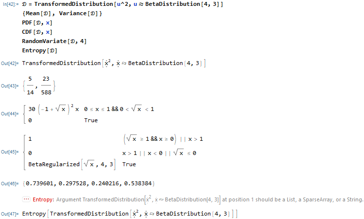
4: Future and other and general tranformations of random variables
Numerical vs Symbolic:


I discussed the following examples on Discourse.
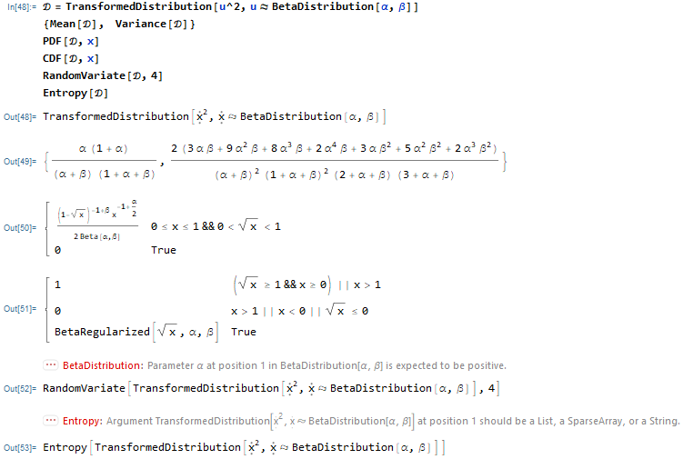
Distributions.jl currently doesn’t operate on transformations of random variables. Mathematica can handle transformations of a distribution when it can solve the problem symbolically.
Now consider the same distribution with symbolic parameters BetaDistribution[α,β]
From paper:
Type hierarchy
- Sampling interface
- Distribution interface and types
R equivalentp-d-q-rin Julia: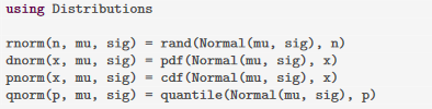
- Distribution fitting and estimation
parametric:fit(D, data)
non-parametric:fit(Histogram, data) - Modeling mixtures of distributions
The table below adds Julia, Mathematica, and Python.
Python: https://github.com/QuantEcon/rvlib
R: https://github.com/alan-turing-institute/distr6
Compare syntax: https://hyperpolyglot.org/scripting
Leave a Comment